Matlab Problems
Mat lab 1:
A free-falling rock is released at an altitude of 50 m. Earth’s gravity g = 9.81 m/s^2 is the only force acting upon the rock. (i.e. no atmospheric drag). Using MATLAB, plot the altitude, velocity, and acceleration as a function of time (4 seconds in 0.05-second steps) in one figure using the “subplot” function. In a second figure plot the velocity as a function of the altitude
Mat lab 2:
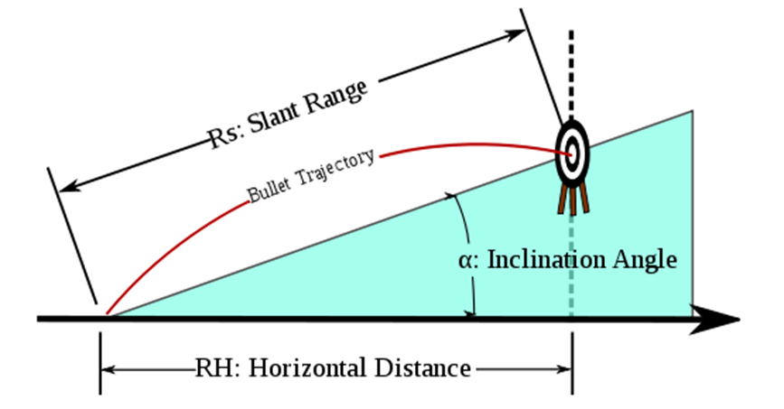
A projectile is shot at an angle of 50 degrees with respect to the horizontal at a velocity of 200 m/s. Earth’s gravity is 9.81 m/s^2. Take the variable x as the range and y as the altitude. Create a MATLAB plot, which plots that trajectory. Now, assume the terrain slopes up by 1 m in y for every 10 m in x. On the same axis, plot the line of the terrain in a different color.
Mat lab 3:
Continuing with the MATLAB problem from Module 2, use a “for” loop or a “while” loop to propagate the projectile in 0.01 second time steps all the way until impact. Mark the impact spot with a marker and display the impact coordinates on the projectile/terrain plot. Label the axes accordingly and give your figure a title. While keeping the initial velocity constant, “experimentally” determine the initial angle of the projectile with respect to the horizontal in order to achieve maximum range. Share that result with your fellow students.
Mat lab 4:
Mat lab 6:
Matlab 7
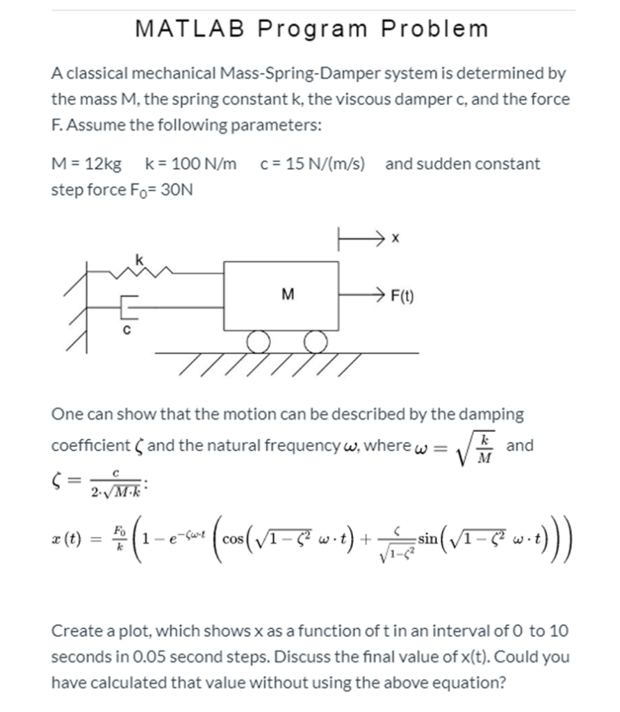
A classical mechanical Mass-Spring-Damper system is determined by the mass M, the spring constant k, the viscous damper c, and the force F. Assume the following parameters:
M = 12kg k = 100 N/m c = 15 N/(m/s) and sudden constant step force F0= 30N
One can show that the motion can be described by the damping coefficient ζ and the natural frequency
ω, where
ω = k M and
ζ = c 2 ⋅ M ⋅ k:
x ( t ) = F 0 k ( 1 − e − ζ ω ⋅ t ( cos ( 1 − ζ 2 ω ⋅ t ) + ζ 1 − ζ 2 sin ( 1 − ζ 2 ω ⋅ t ) ) )
Create a plot, which shows x as a function of t in an interval of 0 to 10 seconds in 0.05 second steps. Discuss the final value of x(t). Could you have calculated that value without using the above equation?
Mat lab 8:
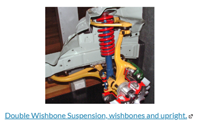
This is a continuation of the discussion during module week 7: In this case, the shock/suspension system of a car needs to be sized. Assume a car with a mass M = 1200 kg having a suspension system, where the overall spring constant k = 48000 N/m. The car hits a bump in the road, which is equivalent to a force of 9000N. Now, take eight different viscous shock absorbers c which ranges between 3000 N/(m/s) and 10000 N/(m/s). Plot the displacements as a function of time and discuss the results with your peers. Also, determine k and c such that the “Overshoot” is below 10% of its final value and the system has settled within 0.33 seconds.