
For sample answers, Whatsapp +91-9976287245
Gradually Varied Flow Profiles and Numerical Solution of
the Kinematic Equations
Objectives
- Evaluate and apply the equations available for the description of open channel flow
- Solve the equations governing unsteady open channel flow
- Apply the equations of unsteady flow to practical flow problems
Rationale
This assignment is based on the material covered in this course. As such you will be directed to
attempt tutorial questions from modules 1-5 before starting this assignment
Important Information
Before starting please review the USQ’s Academic Integrity Policy and Procedure:
“All assessable work in a course is to be the individual student’s own work, unless advised
otherwise in the Course Specification. It is unacceptable for students to share solutions to
assessable work on this Study Desk site, or in any other manner. Violations of this principle
are regarded as Academic Misconduct and will be dealt with under the USQ Academic
Regulations.”
For guidance on what constitutes Academic Misconduct and its various categories, at USQ
refer to the USQ Student Academic Misconduct Policy available at:
http://policy.usq.edu.au/documents/13752PL
Instructions for Submission
Submission for this assignment is in two parts:
- Report introducing the problem, providing background in all relevant theory, descriptions
of methods and equations used and discussion of results. - Electronic copy of all computer code or spreadsheets used so the examiner can validate the
models
The report should be compiled in such a manner that assessment can be completed without access
to the electronic copies of the code/spreadsheet files. It is normal practice to include technical
details (e.g. computer code) as an appendix.
The assignment is to be submitted electronically via study desk. The link is available on the course
studydesk.
Please note that hand written equations within the body of the report are permitted. In many
cases they are preferred as they are simpler to produce and easier to read than poorly set out
computer produced equations
Question 1 – Gradually Varied Flow Profiles
Water is flowing in a long prismatic channel with a triangular cross-section. The side slope of
the cross-section is 1(V):2.5 (H). The channel is constructed of rough gravel for which the
Manning roughness is of 0.025.
The downstream end of the channel contains a weir structure which causes the water level to
rise 0.75 m above the normal flow depth. Take alpha (α) as being 1.0 (1.0).
Your task:
a) Use the direct step method, and the equation below to compute the water surface profile
upstream of the weir.

b) Plot the water depth against distance
c) Plot the longitudinal bed, normal depth, critical depth, water surface and energy line over the
length of this profile. (All on the same set of axis and corrected for height of the bed e.g. Fig
5.22 Chadwick)
d) Include sample hand calculation in the report
Hints:
- The size of the step is up to you.
- Use of computers for this task (Matlab, Excel etc is encouraged)
- When computing the water surface profile you should stop just short of normal depth
- The Froude number and critical depth for a triangular channel are different to that of a
rectangular channel (e.g. need average depth ( y ) instead of max depth ( y ) in R F )
Question 2 – Kinematic Wave Model
Background
You have been asked to investigate the flow behaviour of a large car park subjected to a short
duration high intensity storm rainfall event.
As part of the process you will develop a computer program of the water depths and flow rates
for a specified rainfall pattern. The kinematic wave approximation is a simple form of one
dimensional flow model, which is deemed sufficient for this task.
The Car Park
For study purposes it has been deemed sufficient to represent the behaviour of the car park with
a one dimensional hydraulic model, in effect reducing the two dimensional car park to a unit
flow width running down the predominant slope direction. Basically, you will estimate water
depth and flow rate per unit width at constant interval.
The specifications of the car park are as follows:


Manning n = Based on your research (you must assume appropriate surface materials)
The car park is freely draining at the downstream end.
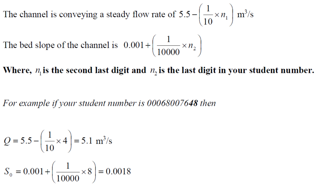
Design Inflow
The model will be used to investigate the flow behaviour subjected to an extreme rainfall
event. An example of such event occurs in Queensland Southeast region in January 2011 (ICA,
2011). For the purpose of this assignment, the inflow at the upstream end of the carpark has
been estimated roughly from rainfall hyetograph as shown in Table 1.
For simplicity it will be assumed in this study that the surface was already saturated at the start
of the storm event and that there is no loss to account.

Your Task
1) Complete the tutorial problems 5.1, 5.2, 5.3 and 5.4 in Module 5. You will find full
solutions of first three questions in the study book that will help you to solve 5.4. The
solution of 5.4 will be used to develop your own computer model.
2) OPTIONAL: If you are not confident about your answer to 5.4 you may submit your
working (formulas/equations) to the examiner using the link provided on studydesk
before proceeding with the numerical scheme. Your examiner will be able to guide you
through.
3) Build your model (using any programming language or spreadsheet) for solving the
kinematic wave equations for computing depth and flow rate resulting from the storm
events. You must configure your model according to the specifications above.
4) Validation is important part for any model development. To validate your mathematical
model, you need to compute the runoff resulting from steady rainfall (assume constant
rainfall depth for sufficient period) and compare results with the analytical results for
steady rainfall. The analytical procedure has been discussed at the end of this problem
(The section Model Validation)
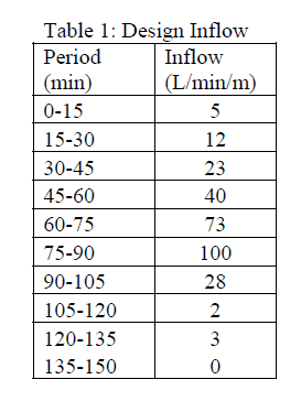
You are required to check all three conditions
5) Modify the model to accommodate the design inflow, which you will use as upstream
boundary condition in the model. The model should run for sufficiently long period to
show the recession in the outflow hydrograph. You don’t need to account lateral inflow
as you may assume that this has been accounted in the given inflow data, which is
deemed acceptable for the purpose of this assignment.
6) Write up all equations, model development, validation, results and discussion in a
report format
Presentation of Results
The final report should include as a minimum:
Introduction and background, a description of the problem
Formulation of the finite difference solution,
Basic description of model;
Validation of the model for a constant slope by:
plot of steady depth profile for a constant lateral inflow of sufficiently long duration, and
comparison of your program output with the results from the analytic solutions of the
kinematic equations given below
Evidence that the Courant condition for stability has been satisfied for both the steady
inflow simulation and the simulation of the example storm.
Plots (for the given variable rainfall) of:
the runoff hydrograph (q vs t) at the lower end of the channel (taken to at least 30 min
after the cessation of rainfall), and
the water surface profile (y vs x) when the discharge from the end of the channel is a
maximum. Also note the time at which this maximum discharge occurs.
Appropriate discussion. Some points that you should cover include:
i. What are your assumptions and how they might impact on the ability of your results
to replicate flow in the real world?
ii. Your results for the runoff hydrograph and depth profiles.
iii. General conclusions of the practical use of your model.
Acknowledgement of any sources of information in a reference list
Model Validation
A useful aide in the validation of your program is to run it with a steady rainfall of duration
sufficiently long for steady state conditions to be reached. Your results for this case can be
compared to the analytic solutions as derived below based on the concept from Stephenson and
Meadows (1986).
For a steady rainfall these are:
Note: In order to use these validations, (particularly 1 & 3) you will need to model a simple plane
surface with a single constant slope and constant Manning roughness subject to a steady
rainfall rate.